With Microsoft Azure, it's easy to create an AI model.

1. Create Studio ML Resource

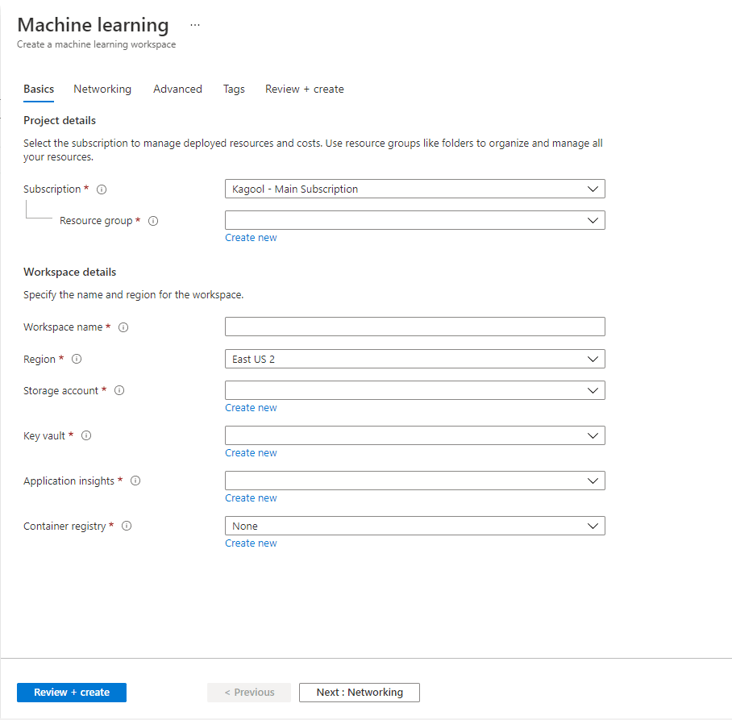
The first thing we need to do is create a ML Studio resource. To do this go to Azure Portal and search for ML Studio. Create a new resource and fill in the details following this Microsoft Guide.

It is a good idea to create a separate storage account for your ML Studio resource.

2. Create a Compute Resource for ML Studio

ML Studio requires a storage account to store Assets and a compute resource to train or inference a model.

During resource creation you should have already created or linked to a storage account.

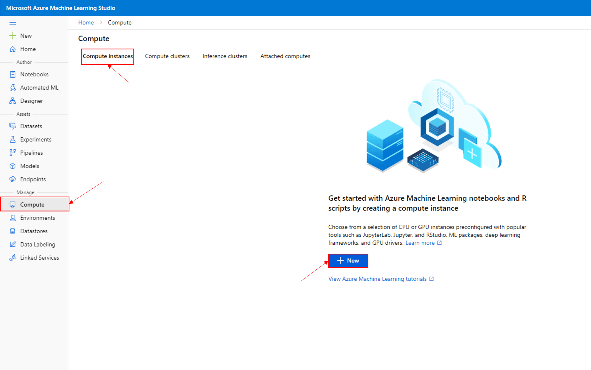
Let’s create a simple compute resource.

As we are doing a single training program that will be computationally inexpensive, we will use a compute instance.

In your ML studio resource go to Compute -> Compute instances -> New

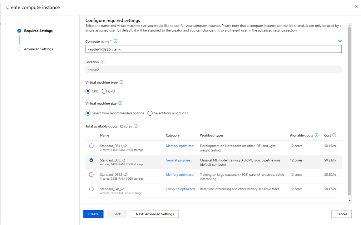
Give your resource a unique name.

Select an appropriate VM. We don’t need anything fancy for this so we will use a Standard_DS3_v2 resource.

Configure any advanced settings you require; I am going to leave as is for the demo.

Press create and wait for the resource state to turn green and say Running.

3. Import the data

We now have our environment to train a simple ML model.

First, let’s import the dataset for training the model into the storage account connected to our ML Studio resource.

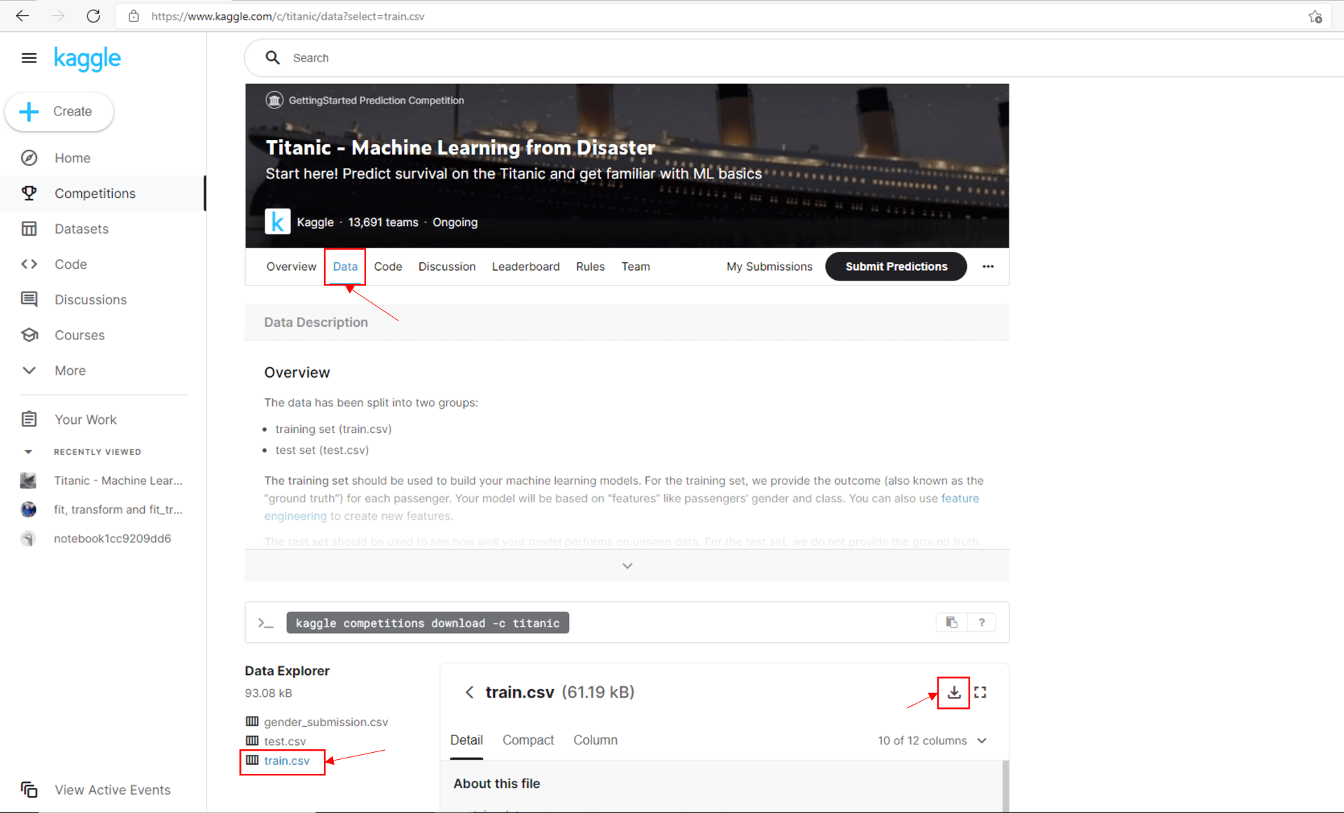
Go to the Kaggle titanic competition page and download the train dataset. We will use this data to train our classification model.

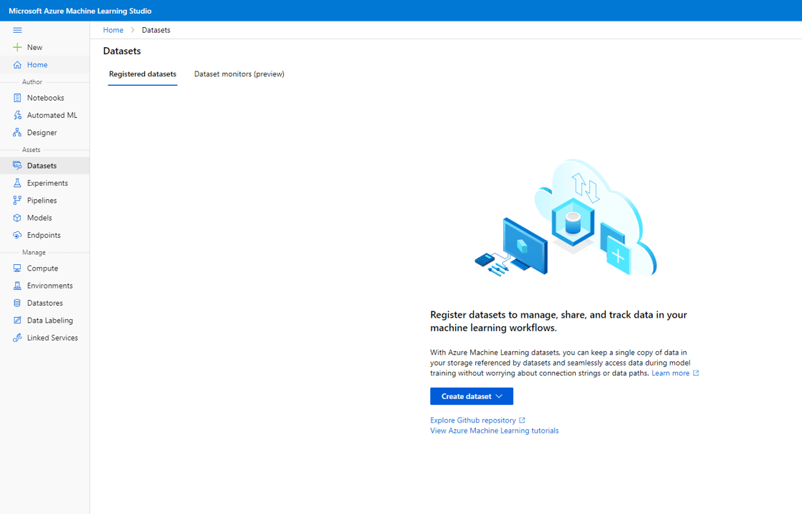
In ML Studio, select Assets -> Datasets -> Registered datasets -> Create dataset

Select from local file.

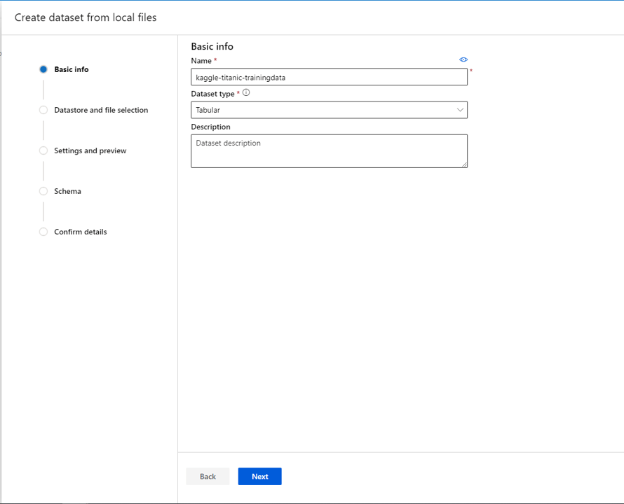
Give the dataset an intuitive name and select Tabular for Dataset type 

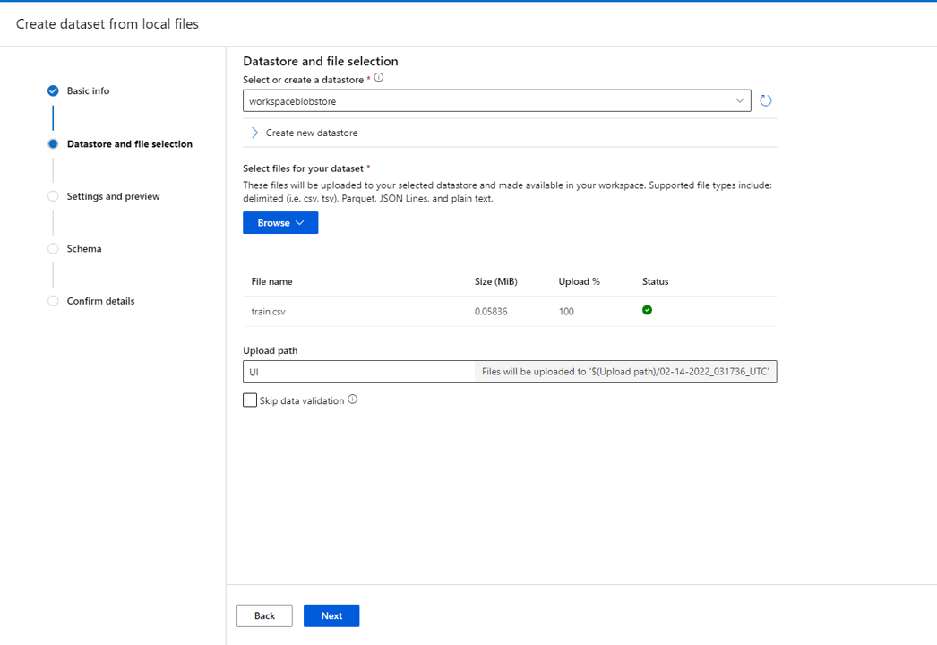
Select next, then select workplaceblobstore as the datastore. This uses the storage account associated to the ML Studio workspace. Under the browse option, attach the train.csv file from your local storage and press next. 

Leave settings and preview as is.

Leave schema as is. We could set it here, but we will set it in the pipeline instead as this makes it easier to change if we make a mistake.

Select next and create the dataset.

4. Create the project pipeline

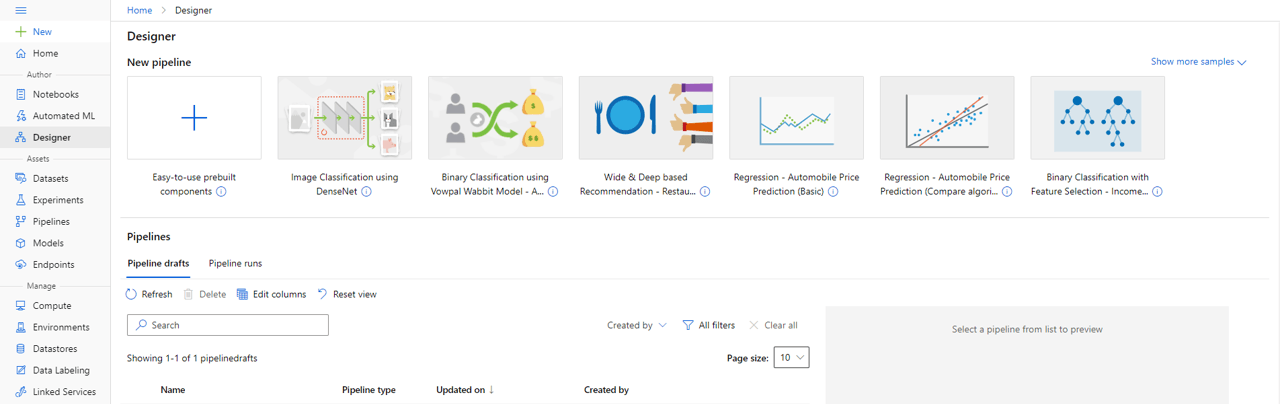
Go to Author -> Designer -> New pipeline -> Easy-to-use prebuilt components 

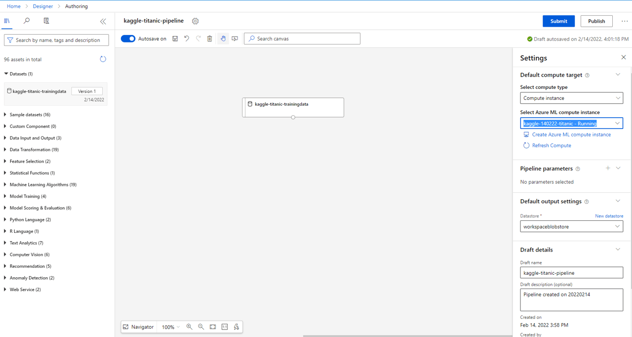
Configure pipeline settings:

• Select the compute resource created earlier
• Set the Draft name to something intuitive
• Under Datasets pull in the training data imported earlier 

5. Clean and prepare the data for training

In its current format the data would not perform very well when training the model. Some columns have data missing, some columns are non-numeric and some columns will bias the model due to their scale. We need to solve all these problems before we can select and train our model.

1. Set column datatypes

First of all, we need to specify the datatype of all the columns and specify which are features and which is the label column.

Integer values:

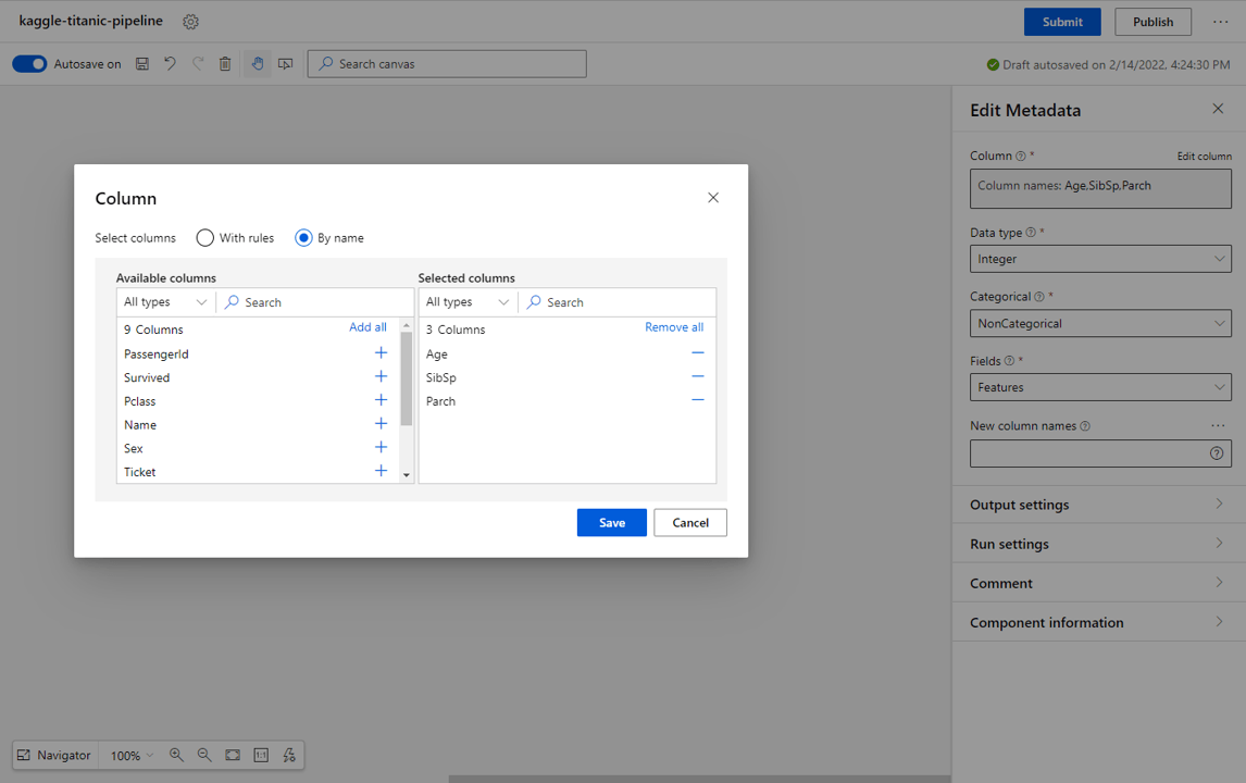
• From the blocks on the left select Edit Metadata.
• Select Edit column from the settings, then select by name in the select columns checkbox.
• Select the Age, SibSp, Parch columns* and select Save.
• In the Edit Metadata settings, set the Data type to Integer, the Categorical type to NonCategorical and the Fields type to Features

String values:

• From the blocks on the left select Edit Metadata.
• Select Edit column from the settings, then select by name in the select columns checkbox.
• Select the PassengerId, Name, Ticket and Cabin* and select Save.
• In the Edit Metadata settings, set the Data type to String, the Categorical type to NonCategorical and the Fields type to Features.

Double values:

• From the blocks on the left select Edit Metadata.
• Select Edit column from the settings, then select by name in the select columns checkbox.
• Select the Fare* and select Save.
• In the Edit Metadata settings, set the Data type to Double, the Categorical type to NonCategorical and the Fields type to Features.

Categorical values:

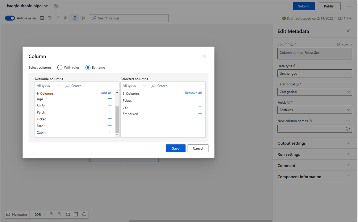
• From the blocks on the left select Edit Metadata.
• Select Edit column from the settings, then select by name in the select columns checkbox.
• Select the Pclass, Sex, Embarked* categories and select Save.
• In the Edit Metadata settings, set the Data type to Unchanged, the Categorical type to Categorical and the Fields type to Features.

Label Values:

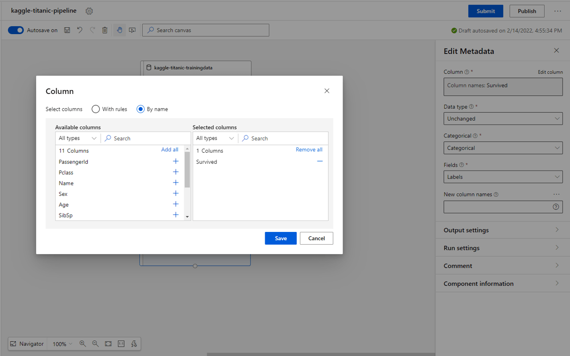
• From the blocks on the left select Edit Metadata.
• Select Edit column from the settings, then select by name in the select columns checkbox.
• Select the Survived* category and select Save.
• In the Edit Metadata settings, set the Data type to Unchanged, the Categorical type to Categorical and the Fields type to Labels.

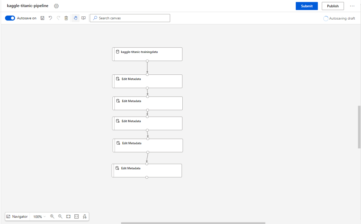
We should now have a pipeline that looks something like this:

*Integer columns should be data where the values follow a sequential pattern of whole integer numbers. Hence PassengerID is not considered an integer type as we cannot say that a value of 2 holds any relationship to a value of 1. String column should be data where there is no relationship between values. Double columns should contain data where the data can be any numerical value and follows a sequential pattern. Categorical columns should contain only entries that match a set of predetermined values. Label columns should be what we are trying to predict. As this is a classification problem, the label is also a categorical type.

2. Select relevant columns

Next, we will select the columns we think are most relevant to train the model. In this process we are going to disregard some columns we have processed in the last step. This may seem like a waste, but it means that if we come back later and decide to use different features (or create new features e.g. PCA) we already have the features formatted.

Drag the Select Columns in Dataset block into the pipeline and attach it to the last Edit Metadata.

• Select Edit column from the settings, then select by name in the select columns checkbox.
• Select the Survived, Pclass, Sex, Age & Fare categories and select Save. 

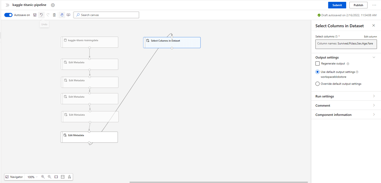
We have chosen these as I am assuming there is a strong correlation between each of these features and the chance of survival. In practice, a better approach would to be explore the relationship of each feature with the label, or to train multiple instances using a variety of labels and assess over a validation dataset. For an introduction into no-code ML, simply taking the above features will suffice (but feel free to explore alternate features, you may get a better model performance!)

3. Clean up missing values

Next, we will clean up any missing values from the dataset.

We can see from the dataset source (Kaggle) that the age column contains missing values.

Pull in the Clean Missing Data block and attach Age column. 

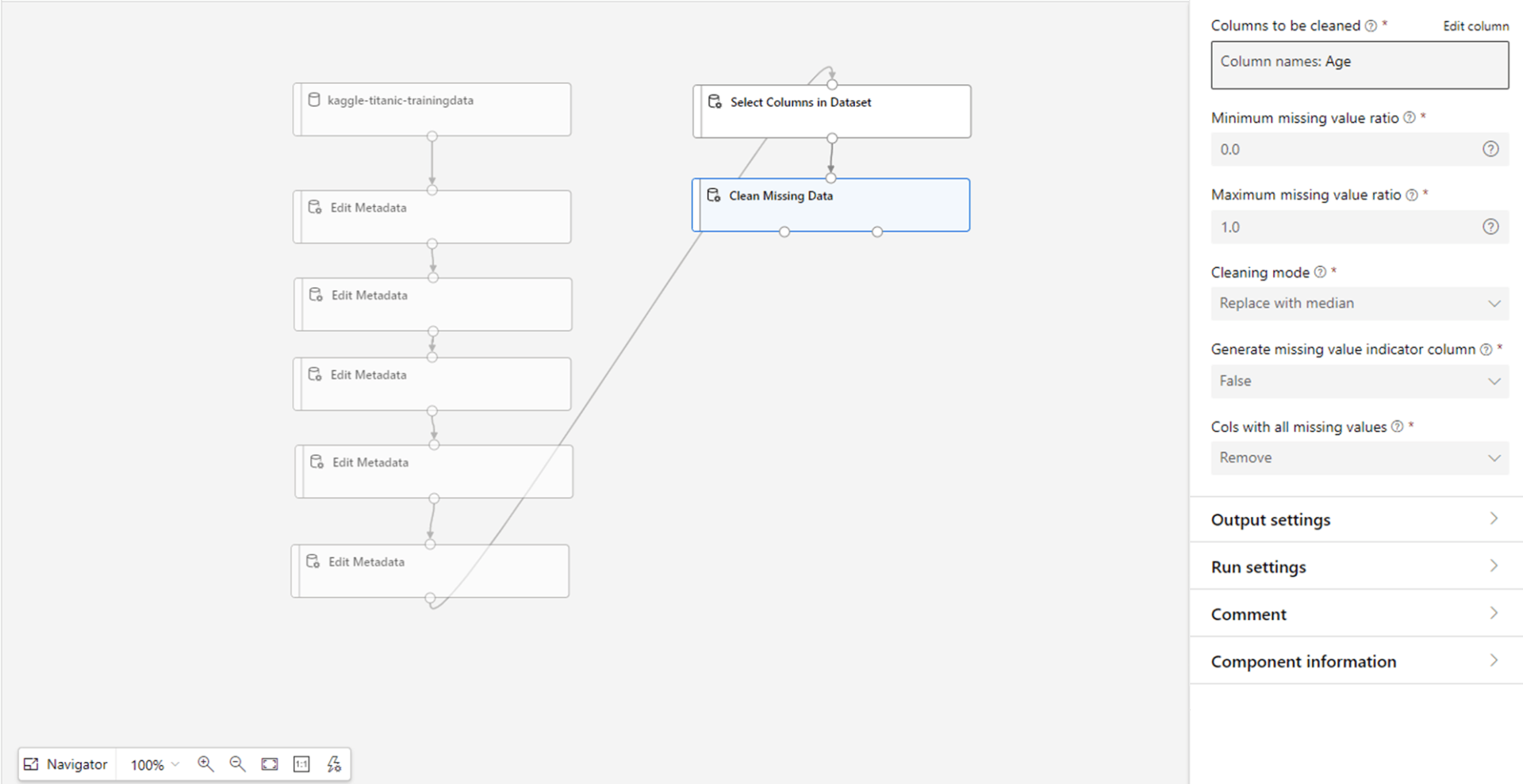
• Leave ratios as they are (we want to replace all missing values) and set the Cleaning mode to replace with median. This will replace any missing values with the median value for the entire column.
• Leave the generate missing value indicator column as false.

4. Convert the categorical columns into binary columns

Now we will sort out the categorical columns. Most ML models can’t handle categorical inputs and so we need to format it into a method that they can understand. Azure ML does this by converting each categorical value into its own binary column. For example, the Gender column would become 2 new columns: Male and Female, each with a value of 1 for true. This type of encoding is referred to as one-hot-encoding.

In the pipeline, pull in the Convert to Indicator Values block and select the Pclass, Sex columns. 

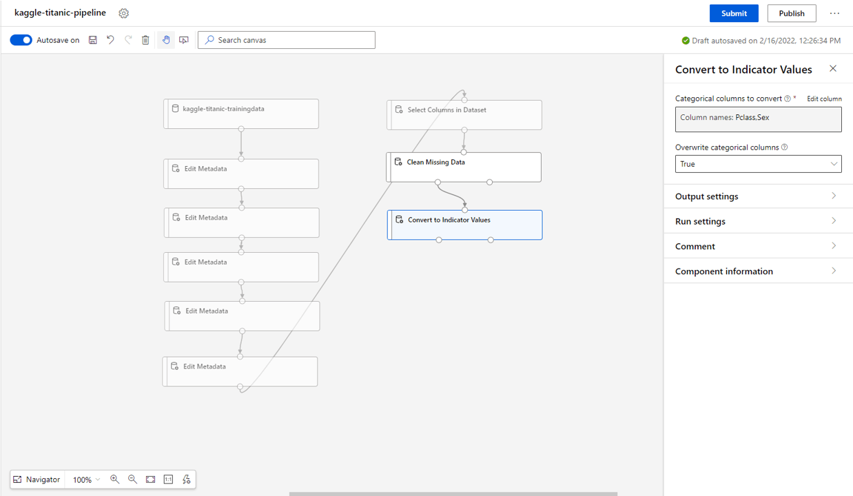
• Select true for overwrite categorical columns as we do not want to retain the original columns after transform (we only want the encoded columns).

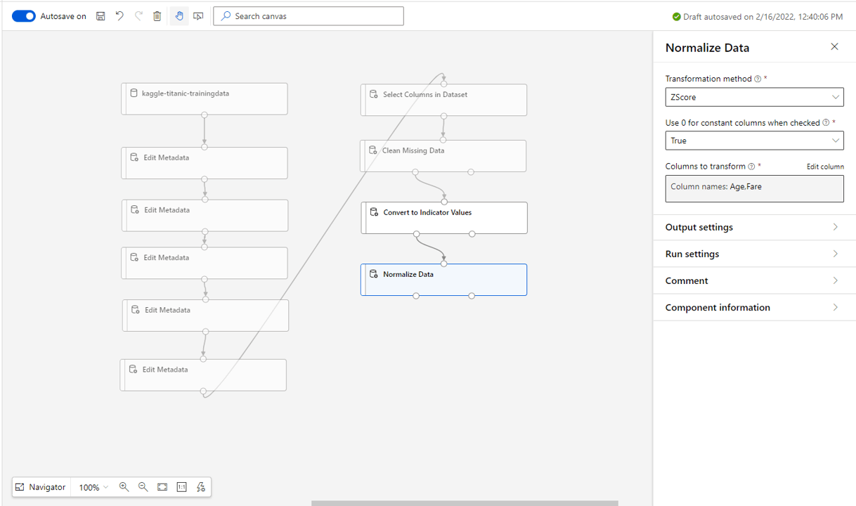
5. Normalise the data

Finally, we will normalise the data. The scale of some features (e.g. Age) is much larger than other features (e.g. Sex – Male), which can result in a biased model that puts more weight on certain fields leading to poor performance.

To counter that we normalise all fields so that they are on a similar scale but retain their statistical variance.

• Drag in the Normalise Data block and select the Age and Fare columns.
• We will leave the transformation method as Zscore.

(Another popular method is MinMax, however this can lead to single outlier records having a major impact on the scaling and affecting the weight the model places on the feature.)

6. Train the model

Hurray! We now have a nice clean dataset that we are ready to use to train a model. #

1. Split dataset into training, validation and testing sets

First, we need to split the dataset into a training, validation and testing set.

• The training set will be used to train various models with various hyperparameter values.
• The validation set will be used to choose which model is best.
• The test set will be used to gain a final performance score for that best model.

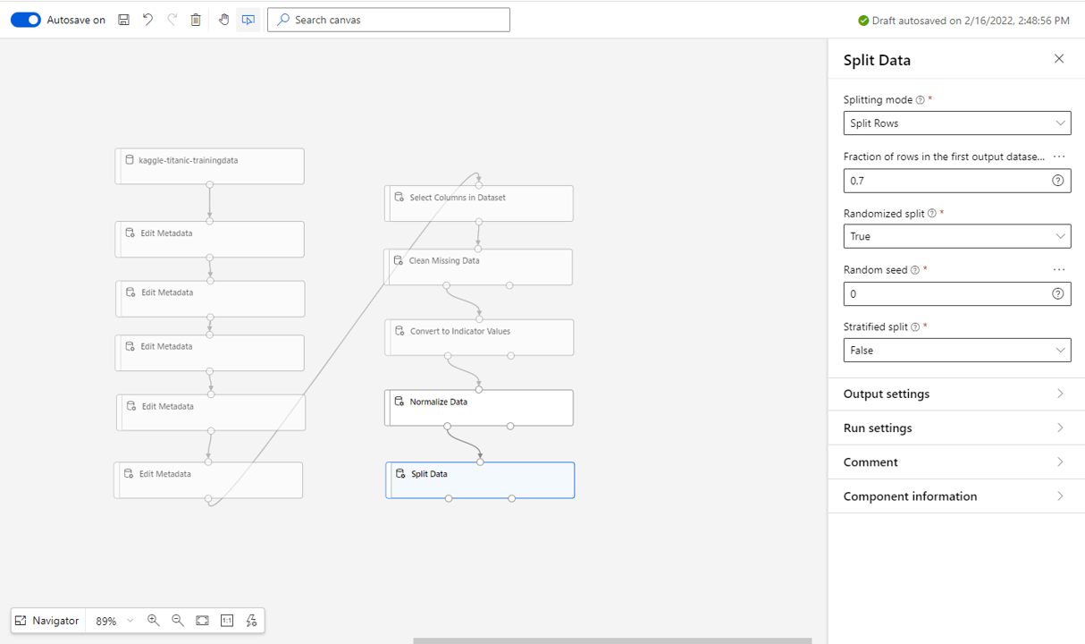
We will randomly select 70% of our data to train & validate the model and 30% to test the best model.

• Drag in the Split Data block and connect to the normalised data.
• Leave the splitting mode to split rows and set the fraction of rows to 0.7 (70%).
• Make sure the Randomised Split is set to True. 
  
• This will output the training and validation set to the left node and the testing set to the right. 
  

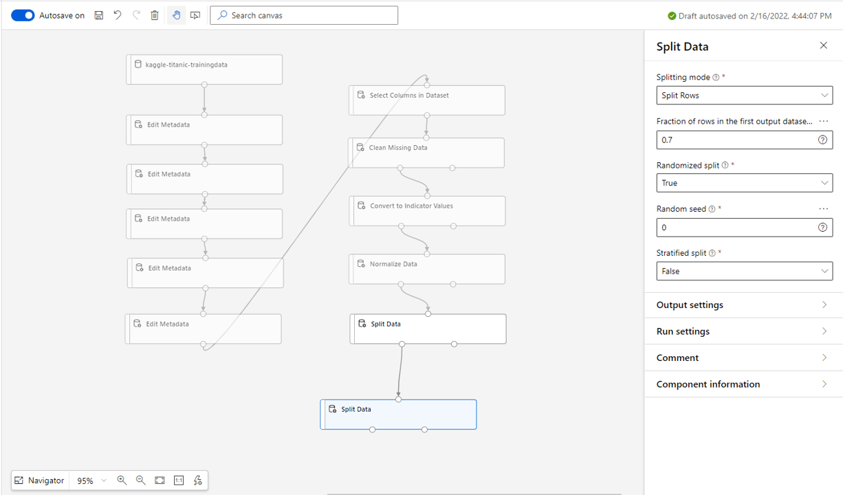
• Drag in another Split Data block and connect to the training output from the first split data block.
• Leave the splitting mode to split rows and set the fraction of rows to 0.7 (70%).
• Make sure the Randomised Split is set to True.
• This will output the training set to the left node and the validation set to the right. 

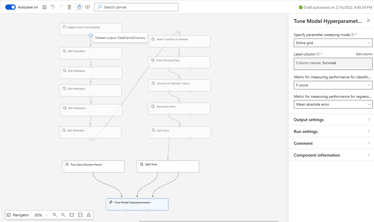
2. Select the type of model to train

We are performing a two-class classification problem (survived or did not survive) so we will select a Two-Class Decision Forest Block and drag it into the pipeline.

You could try any alternative two-class model, or even train multiple and validate the best performing model using the validation set.

We will not set any of the model hyperparameters (e.g. number of decision trees) as we will automate training multiple instances of the model with various hyperparameters, and select which one performs best on the validation set.



Next pull in the Tune Model Hyperparameters block. This performs the process listed above. Attach the model, training data and validation data to the nodes in that order as shown. Set the sweeping mode to Entire grid and the Metric for measuring performance for classification to F-score. Set the Label Column to Survived as this is what we are predicating. 

7. Assess the model

Now, when the pipeline runs, we will have a trained model that we can use. Once trained, we will need to assess its performance on the testing data (which it hasn’t seen before).



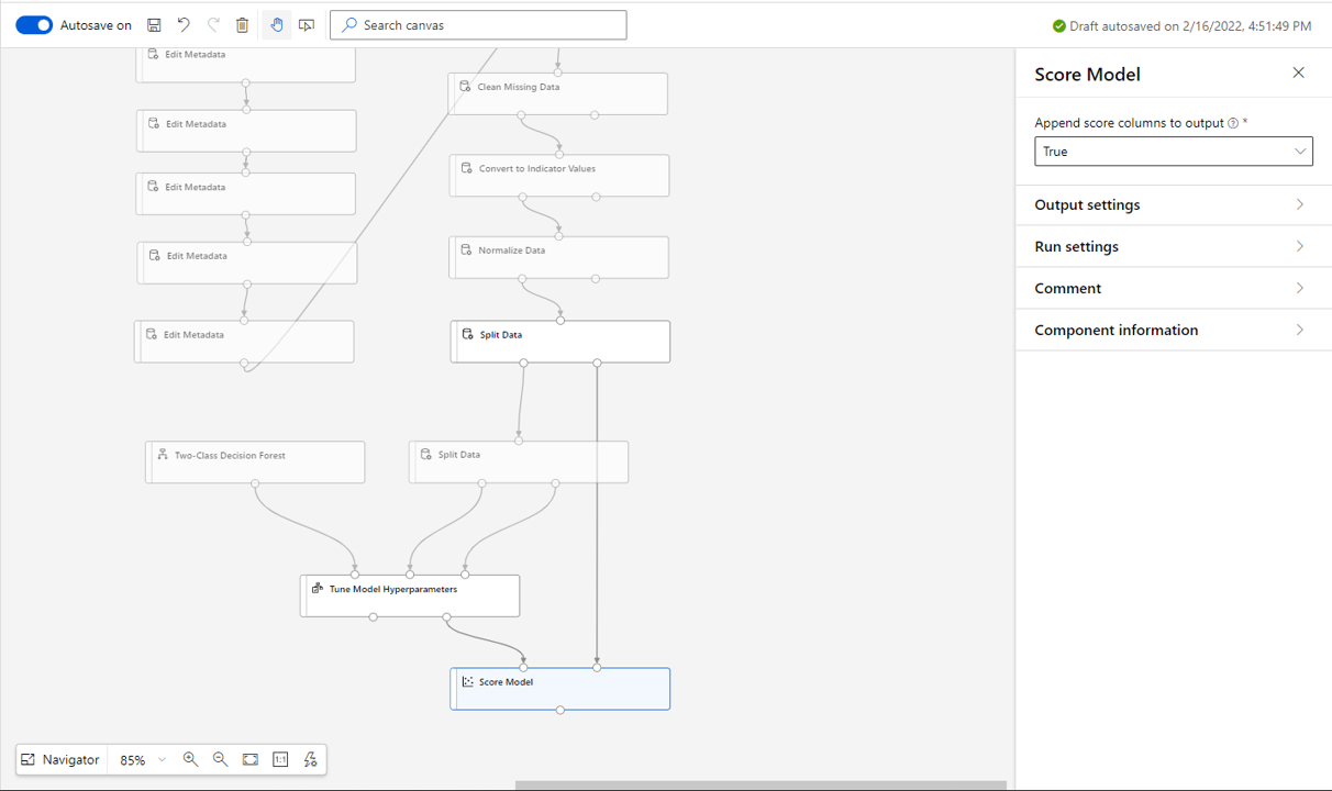
Pull in a Score Model block from the right and connect the tuned model and test set as shown. We don’t need to make any settings changes here.



Pull in a Evaluate Model block and attach the Score Model output as seen below.

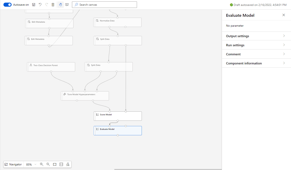
We are now ready to run the pipeline and see what we get.

8. Run the pipeline

Make sure your compute instance created earlier is running.

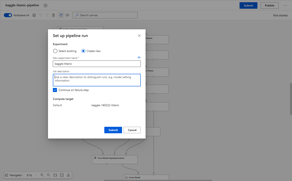
Select Submit from the top then select create new experiment. Give the experiment an intuitive name and press Submit.



The pipeline will begin running. Wait for all tasks to complete.

Now let’s see how our model performed.

• Click on the evaluate model block.
• Select Outputs + logs and click the small graph icon.
• From here we can analyse the results of the model.

9. Analysing performance

Assessing the performance of a classifier is often highly dependent on the scenario.

For example, if we were diagnosing whether someone should be screened for cancer (label) based on symptoms (features), sending a few extra people (false positives) to be tested when they shouldn’t is not too much of a problem. But we definitely don’t want to accidently refuse someone screening when they should be (false negative).

This complexity is well documented and there are plenty of other online resources on choosing the best performance criteria, so we won’t dive into that here.

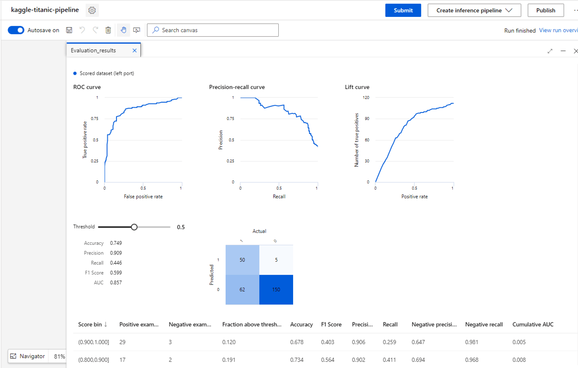
For our classifier we will assess the performance based on accuracy. This is the fraction of instances that were correctly classified.

We can see that we have an accuracy of about 75%, which is not bad for a simple classifier.

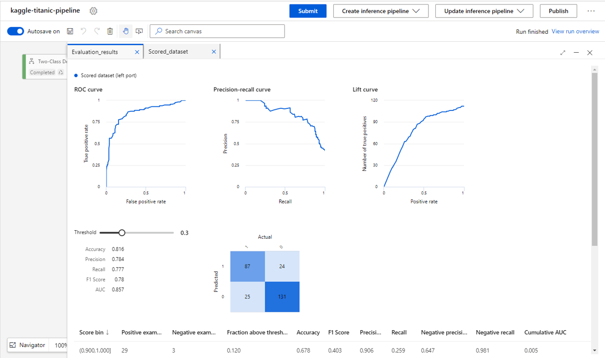
We can see a threshold bar above the results. This lets us specify the confidence at which an instance will be classified as having survived.

With a value of 0.5 the classifier will set any instances that it believes have an above 50% chance of surviving to survived.

Lets drop the value to 0.3 (30+ % chance of survival will survive) and see what happens {pic 9.1}

Notice that our overall accuracy increase now to 82% & our false negative rate drops, but we now have a higher false positive rate

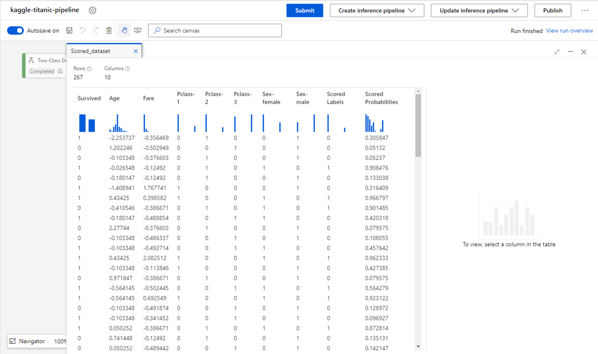
Finally let’s have a look at the raw data.

• Clicking on the Score Model then Output and logs and finally the graph icon we can view the tabulated results (below).
• Here we can see for the true result (Survived), the predicted result (Scored Labels) and the probabilities of those predictions (Scored Probabilities) for each instance in the training set.

10. All done!

And that’s it! We have now used the pipeline designer in ML studio to build a no-code classifier to predict whether someone would survive on the titanic.

To summarise the steps:

• First, we created a ML Studio resource and set up its dependencies.
• We then imported the dataset and created a pipeline project.
• After that we cleaned the data and got it ready for model training.
• Then we trained a random forest classifier.
• And finally, we analysed the model performance.

We have just seen the tip of the iceberg (pun intended…) of what Azure ML Studio can offer.

Once you have a basic classifier trained, explore ways of improving your model performance and let us know how it goes on LinkedIn. A few ideas:

• Try different models
• Explore PCA and what the best number of features could be
• Try an ensemble classifier based upon different classifiers

Good luck!